Concept explainers
Videos
In working further with the problem of exercise 4, statisticians suggested the use of the following curvilinear estimated regression equation.
- a. Use the data of exercise 4 to compute the coefficients of this estimated regression equation.
- b. Using α = .01, test for a significant relationship.
- c. Estimate the traffic flow in vehicles per hour at a speed of 38 miles per hour.
4. A highway department is studying the relationship between traffic flow and speed. The following model has been hypothesized.
where
y = traffic flow in vehicles per hour
x = vehicle speed in miles per hour
The following data were collected during rush hour for six highways leading out of the city.
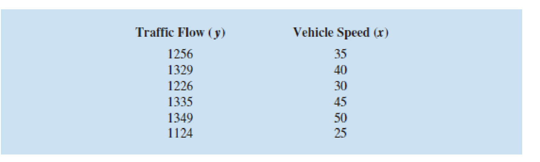
- a. Develop an estimated regression equation for the data.
- b. Using α = .01, test for a significant relationship.
Want to see the full answer?
Check out a sample textbook solution
Chapter 16 Solutions
Modern Business Statistics with Microsoft Office Excel (with XLSTAT Education Edition Printed Access Card) (MindTap Course List)


- The following table provides values of the function f(x,y). However, because of potential; errors in measurement, the functional values may be slightly inaccurately. Using the statistical package included with a graphical calculator or spreadsheet and critical thinking skills, find the function f(x,y)=a+bx+cy that best estimate the table where a, b and c are integers. Hint: Do a linear regression on each column with the value of y fixed and then use these four regression equations to determine the coefficient c. x y 0 1 2 3 0 4.02 7.04 9.98 13.00 1 6.01 9.06 11.98 14.96 2 7.99 10.95 14.02 17.09 3 9.99 13.01 16.01 19.02arrow_forwardDoes Table 1 represent a linear function? If so, finda linear equation that models the data.arrow_forwardOlympic Pole Vault The graph in Figure 7 indicates that in recent years the winning Olympic men’s pole vault height has fallen below the value predicted by the regression line in Example 2. This might have occurred because when the pole vault was a new event there was much room for improvement in vaulters’ performances, whereas now even the best training can produce only incremental advances. Let’s see whether concentrating on more recent results gives a better predictor of future records. (a) Use the data in Table 2 (page 176) to complete the table of winning pole vault heights shown in the margin. (Note that we are using x=0 to correspond to the year 1972, where this restricted data set begins.) (b) Find the regression line for the data in part ‚(a). (c) Plot the data and the regression line on the same axes. Does the regression line seem to provide a good model for the data? (d) What does the regression line predict as the winning pole vault height for the 2012 Olympics? Compare this predicted value to the actual 2012 winning height of 5.97 m, as described on page 177. Has this new regression line provided a better prediction than the line in Example 2?arrow_forward
- If your graphing calculator is capable of computing a least-squares sinusoidal regression model, use it to find a second model for the data. Graph this new equation along with your first model. How do they compare?arrow_forwardThe following fictitious table shows kryptonite price, in dollar per gram, t years after 2006. t= Years since 2006 0 1 2 3 4 5 6 7 8 9 10 K= Price 56 51 50 55 58 52 45 43 44 48 51 Make a quartic model of these data. Round the regression parameters to two decimal places.arrow_forwardFor the following exercises, consider the data in Table 5, which shows the percent of unemployed in a city ofpeople25 years or older who are college graduates is given below, by year. 41. Based on the set of data given in Table 7, calculatethe regression line using a calculator or othertechnology tool, and determine the correlationcoefficient to three decimal places.arrow_forward
- ) A real estate magazine reported the results of a regression analysis designed to predict theprice (y), measured in dollars, of residential properties recently sold in a northern Virginiasubdivision. One independent variable used to predict sale price is GLA, gross living area(x), measured in square feet. Data for 157 properties were used to fit the model,? = β0 + β1x.The results of the simple linear regression are provided below.y = 96,600 +22.5x s = 6500 r2 = -0.77 t = 6.1 (for testing β1)Interpret the estimate of β0 the y-intercept of the line.a. About 95% of the observed sale prices fall within $96,600 of the least squares line.b. There is no practical interpretation, since a gross living area of 0 is a nonsensicalvalue.c. All residential properties in Virginia will sell for at least $96,600.d. For every 1-sq ft. increase in GLA, we expect a property's sale price to increase$96,600.arrow_forwardThe estimated regression equation for a model involving two independent variables and 10 observations follows. ŷ = 32.4394 + 0.5695x1 + 0.7347x2 a. Interpret b1 and b2 in this estimated regression equation (to 4 decimals). b. Estimate y when x1 = 180 and x2 = 310 (to 3 decimals).arrow_forwardA kinesiology major wanted to predict VO2max based on the one-mile run. To develop the regression equation, she obtained VO2max values (ml/kg/min) in the exercise physiology laboratory on 18 students. Two days later, she measured the same 18 students on the one-mile run with scores reported as total time in seconds. The data are as follows: X Y r = -.94 Subject One-mile run time (seconds) VO2 max (ml/kg/min) 1 250 60.3 2 315 57.2 3 420 55.4 4 410 51.4 5 436 52.5 6 511 45.6 7 460 38.4 8 510 41.5 9 530 39.6 10 586 33.2 11 591 37.7 12 600 40.1 13 626 32.0 14 643 35.4 15 650 33.7 16 675 35.9 17 710 27.4 18 720 25.3 Calculate means for one-mile run and VO2 = = Calculate the slope of the line (b) using this formula: Interpret your answer: Calculate the y-intercept (a) using this formula: What is…arrow_forward
- 2. A sample of small cars was selected to attempt to use the horsepower (x) in hp of the car to predict the fuel efficiency (y) in miles per gallon. A researcher fitted a linear regression model. ŷ-44.0 -0.150x a) Interpret the slope of the regression line. b) Find the predicted fuel efficiency for a horsepower of 150 hp? c) If the fuel efficiency for a car of horsepower of 150hp had an actual fuel efficiency of 25mpg, what is the residual (error) for this car? d) Calculate the correlation coefficient. e) What is the strength of the correlation coefficient? R²=68% f) Interpret the y-intercept.arrow_forwardAn agent for a real estate company in a large city would like to be able to predict the monthly rental cost for apartments, based on the size of the apartment, as defined by square footage. A sample of eight apartments in a neighborhood was selected, and the information gathered revealed the data shown below. For these data, the regression coefficients are bo = 212.5651 and b, = 0.9701. Complete parts (a) through (d). Monthly Rent ($) 875 1,500 800 1,600 1,950 950 1,700 1,250 O Size (Square Feet) 800 1,300 1,050 1,100 1,900 750 1,350 950 - measures the proportion of variation in monthly rent that can be explained by the variation in apartment size. b. Determine the standard error of the estimate, Svx. Syx = (Round to three decimal places as needed.)arrow_forwardThe owner of a movie theater company used multiple regression analysis to predict gross revenue (y) as a function of television advertising (x,) and newspaper advertising (x,). The estimated regression equation was ý = 82.3 + 2.29x, + 1.90x2. The computer solution, based on a sample of eight weeks, provided SST = 25.1 and SSR = 23.415. (a) Compute and interpret R? and R 2. (Round your answers to three decimal places.) The proportion of the variability in the dependent variable that can be explained by the estimated multiple regression equation is 653 x . Adjusting for the number of independent variables in the model, the proportion of the variability in the dependent variable that can be explained by the estimated multiple regression equation is (b) When television advertising was the only independent variable, R2 = 0.653 and R,2 = 0.595. Do you prefer the multiple regression results? Explain. Multiple regression analysis (is preferred since both R2 and R.2 show an increased v v…arrow_forward
 College AlgebraAlgebraISBN:9781305115545Author:James Stewart, Lothar Redlin, Saleem WatsonPublisher:Cengage Learning
 Calculus For The Life SciencesCalculusISBN:9780321964038Author:GREENWELL, Raymond N., RITCHEY, Nathan P., Lial, Margaret L.Publisher:Pearson Addison Wesley,
 Algebra and Trigonometry (MindTap Course List)AlgebraISBN:9781305071742Author:James Stewart, Lothar Redlin, Saleem WatsonPublisher:Cengage Learning
 Functions and Change: A Modeling Approach to Coll...AlgebraISBN:9781337111348Author:Bruce Crauder, Benny Evans, Alan NoellPublisher:Cengage Learning
 Trigonometry (MindTap Course List)TrigonometryISBN:9781305652224Author:Charles P. McKeague, Mark D. TurnerPublisher:Cengage Learning