
Concept explainers
Videos
In a simulation of 30 mobile computer networks, the average speed, pause time, and number of neighbor were measured. A “neighbor” is a computer within the transmission
- a. Fit the model with Neighbors as the dependent variable, and independent variables Speed, Pause, Speed,·Pause, Speed2, and Pause2.
- b. Construct a reduced model by dropping any variables whose P-values are large, and test the plausibility of the model with an F test.
- c. Plot the residuals versus the fitted values for the reduced model. Are there any indications that the model is inappropriate? If so, what are they?
- d. Someone suggests that a model containing Pause and Pause2 as the only dependent variables is adequate. Do you agree? Why or why not?
- e. Using a best subsets software package, find the two models with the highest R2 value for each model size from one to five variables. Compute Cp and adjusted R2 for each model.
- f. Which model is selected by minimum Cp? By adjusted R2? Are they the same?
a.
Construct a multiple linear regression model with neighbor as the dependent variable, speed, pause,
Answer to Problem 5SE
A multiple linear regression model for the given data is:
Explanation of Solution
Calculation:
The data represents the values of the variables number of neighbors, average speed and pause time for a simulation of 30 mobile network computers.
Multiple linear regression model:
A multiple linear regression model is given as
Let
Regression:
Software procedure:
Step by step procedure to obtain regression using MINITAB software is given as,
- Choose Stat > Regression > General Regression.
- In Response, enter the numeric column containing the response data Y.
- In Model, enter the numeric column containing the predictor variables X1, X2, X1*X2, X1*X1 and X2*X2.
- Click OK.
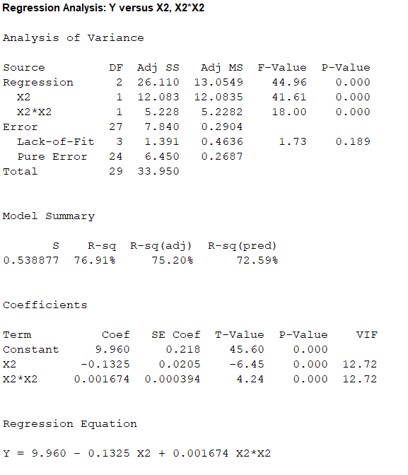
Output obtained from MINITAB is given below:
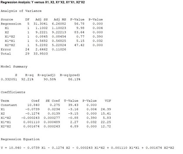
The ‘Coefficient’ column of the regression analysis MINITAB output gives the slopes corresponding to the respective variables stored in the column ‘Term’.
A careful inspection of the output shows that the fitted model is:
Hence, the multiple linear regression model for the given data is:
b.
Construct a reduced model by dropping the variables with large P- values.
Check whether the reduced model is plausible or not.
Answer to Problem 5SE
A multiple linear regression model for the given data is:
Yes, there is enough evidence to conclude that the reduced model is plausible.
Explanation of Solution
Calculation:
From part (a), it can be seen that the ‘P’ column of the regression analysis MINITAB output gives the slopes corresponding to the respective variables stored in the column ‘Term’.
By observing the P- values of the MINITAB output, it is clear that the largest P-value is 0.390 corresponding to the predictor variable
Now, the new regression has to be fitted after dropping the predictor variable
Regression:
Software procedure:
Step by step procedure to obtain regression using MINITAB software is given as,
- Choose Stat > Regression > General Regression.
- In Response, enter the numeric column containing the response data Y.
- In Model, enter the numeric column containing the predictor variables X1, X2, X1*X1 and X2*X2.
- Click OK.
Output obtained from MINITAB is given below:
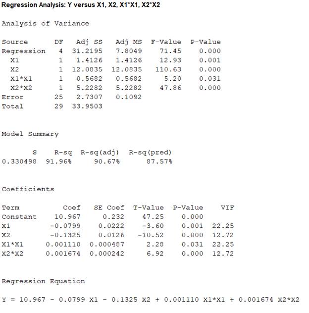
The ‘Coefficient’ column of the regression analysis MINITAB output gives the slopes corresponding to the respective variables stored in the column ‘Term’.
A careful inspection of the output shows that the fitted model is:
Hence, the multiple linear regression model for the given data is:
The full model is,
The reduced model is,
The test hypotheses are given below:
Null hypothesis:
That is, the dropped predictor of the full model is not significant to predict y.
Alternative hypothesis:
That is, the dropped predictor of the full model is significant to predict y.
Test statistic:
Where,
n represents the total number of observations.
p represents the number of predictors on the full model.
k represents the number of predictors on the reduced model.
From the obtained MINITAB outputs, the value of error sum of squares for full model is
The total number of observations is
Number of predictors on the full model is
Degrees of freedom of F-statistic for reduced model:
In a reduced multiple linear regression analysis, the F-statistic is
In the ratio, the numerator is obtained by dividing the quantity
Thus, the degrees of freedom for the F-statistic in a reduced multiple regression analysis are
Hence, the numerator degrees of freedom is
Test statistic under null hypothesis:
Under the null hypothesis, the test statistic is obtained as follows:
Thus, the test statistic is
Since, the level of significance is not specified. The prior level of significance
P-value:
Software procedure:
- Choose Graph > Probability Distribution Plot choose View Probability > OK.
- From Distribution, choose F, enter 1 in numerator df and 24 in denominator df.
- Click the Shaded Area tab.
- Choose X-Value and Right Tail for the region of the curve to shade.
- Enter the X-value as 0.76638.
- Click OK.
Output obtained from MINITAB is given below:
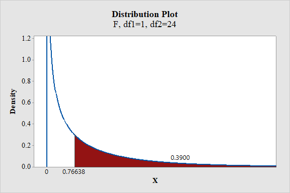
From the output, the P- value is 0.39.
Thus, the P- value is 0.39.
Decision criteria based on P-value approach:
If
If
Conclusion:
The P-value is 0.39 and
Here, P-value is greater than the
That is
By the rejection rule, fail to reject the null hypothesis.
Hence, there is sufficient evidence to conclude that the dropped predictor variable is not significant to predict the response variable y.
Thus, the reduced model is useful than the full model to predict the response variable y.
c.
Plot the residuals versus fitted line plot for the reduced model.
Check whether the model is appropriate.
Answer to Problem 5SE
Residual plot:
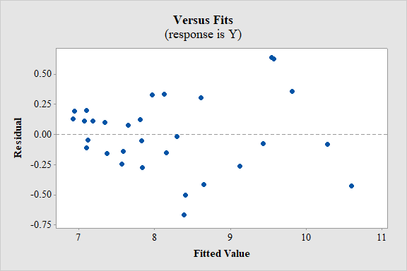
Yes, the model seems to be appropriate.
Explanation of Solution
Calculation:
Residual plot:
Software procedure:
Step by step procedure to obtain regression using MINITAB software is given as,
- Choose Stat > Regression > General Regression.
- In Response, enter the numeric column containing the response data Y.
- In Model, enter the numeric column containing the predictor variables X1, X2, X1*X1 and X2*X2.
- In Graphs, Under Residuals for plots, select Regular.
- Under Residual plots select box Residuals versus fits.
- Click OK.
Conditions for the appropriateness of regression model using the residual plot:
- The plot of the residuals vs. fitted values should fall roughly in a horizontal band contended and symmetric about x-axis. That is, the residuals of the data should not represent any bend.
- The plot of residuals should not contain any outliers.
- The residuals have to be scattered randomly around “0” with constant variability among for all the residuals. That is, the spread should be consistent.
Interpretation:
In residual plot there is high bend or pattern, which can violate the straight line condition and there is change in the spread of the residuals from one part to another part of the plot.
However, it is difficult to determine about the violation of the assumptions without the data.
Thus, the model seems to be appropriate.
d.
Check whether the model with only two dependent variables
Answer to Problem 5SE
No, the model with only two dependent variables
Explanation of Solution
Calculation:
Regression:
Software procedure:
Step by step procedure to obtain regression using MINITAB software is given as,
- Choose Stat > Regression > General Regression.
- In Response, enter the numeric column containing the response data Y.
- In Model, enter the numeric column containing the predictor variables X2 and X2*X2.
- Click OK.
Output obtained from MINITAB is given below:
The ‘Coefficient’ column of the regression analysis MINITAB output gives the slopes corresponding to the respective variables stored in the column ‘Term’.
A careful inspection of the output shows that the fitted model is:
Hence, the multiple linear regression model for the given data is:
The full model is,
The reduced model is,
The test hypotheses are given below:
Null hypothesis:
That is, the dropped predictors of the full model are not significant to predict y.
Alternative hypothesis:
That is, at least one of the dropped predictors of the full model are significant to predict y.
Test statistic:
Where,
n represents the total number of observations.
p represents the number of predictors on the full model.
k represents the number of predictors on the reduced model.
From the obtained MINITAB outputs, the value of error sum of squares for full model is
The total number of observations is
Number of predictors on the full model is
Degrees of freedom of F-statistic for reduced model:
In a reduced multiple linear regression analysis, the F-statistic is
In the ratio, the numerator is obtained by dividing the quantity
Thus, the degrees of freedom for the F-statistic in a reduced multiple regression analysis are
Hence, the numerator degrees of freedom is
Test statistic under null hypothesis:
Under the null hypothesis, the test statistic is obtained as follows:
Thus, the test statistic is
Since, the level of significance is not specified. The prior level of significance
P-value:
Software procedure:
- Choose Graph > Probability Distribution Plot choose View Probability > OK.
- From Distribution, choose F, enter 3 in numerator df and 24 in denominator df.
- Click the Shaded Area tab.
- Choose X-Value and Right Tail for the region of the curve to shade.
- Enter the X-value as 15.702.
- Click OK.
Output obtained from MINITAB is given below:
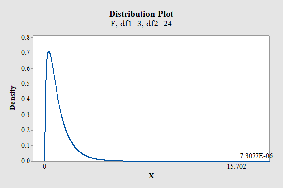
From the output, the P- value is
Thus, the P- value is
Decision criteria based on P-value approach:
If
If
Conclusion:
The P-value is
Here, P-value is less than the
That is
By the rejection rule, reject the null hypothesis.
Hence, there is sufficient evidence to conclude that at least one of the dropped predictors of the full model are significant to predict y.
Thus, the model with only two dependent variables
e.
Find the two models with the highest
Obtain the values of mallows
Answer to Problem 5SE
The two models with the highest
First model with
The values of M Mallows’
| Predictor variables | Mallows’ | Adjusted |
| 92.5 | 60.1 | |
| 97 | 58.6 | |
| 47.1 | 75.2 | |
| 53.3 | 73 | |
| 7.9 | 89.2 | |
| 15.5 | 86.4 | |
| 4.8 | 90.7 | |
| 9.2 | 89 | |
| 6 | 90.6 |
Explanation of Solution
Calculation:
Coefficient of multiple determination
The coefficient of multiple determination,
The subset with larger
Regression:
Software procedure:
Step by step procedure to obtain regression using MINITAB software is given as,
- Choose Stat > Regression > Regression> Best subsets.
- In Response, enter the numeric column containing the response data Y.
- In Model, enter the numeric column containing the predictor variables X1, X2, X1*X2, X1*X1 and X2*X2.
- Click OK.
Output obtained from MINITAB is given below:
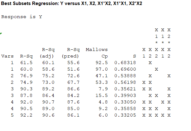
For the one predictor case, the highest value of
For the two predictor case, the highest value of
For the three predictor case, the highest value of
For the four predictor case, the highest value of
For the five predictor case, the value of
The value of
Thus, depending upon the factors affecting the analysis it would be most preferable to use the regression equation corresponding to the predictors
The second highest value of
That is, 90.6 and 90.3 are not much distinct.
Therefore, the model with
Thus, the two best models are:
First model with
From the accompanying MINITAB output, the values of Mallows’
| Predictor variables | Mallows’ | Adjusted |
| 92.5 | 60.1 | |
| 97 | 58.6 | |
| 47.1 | 75.2 | |
| 53.3 | 73 | |
| 7.9 | 89.2 | |
| 15.5 | 86.4 | |
| 4.8 | 90.7 | |
| 9.2 | 89 | |
| 6 | 90.6 |
f.
Select the variables for the model, using the Mallows’
Check whether both the models are same.
Answer to Problem 5SE
The variables for the model using the Mallows’
The variables for the model using the adjusted-
Yes, both the models are same.
Explanation of Solution
Mallows’
An important utility of the Mallows’
Mallows’
The predictor with the lowest value of
From part (e), the values of Mallows’
| Predictor variables | Mallows’ | Adjusted |
| 92.5 | 60.1 | |
| 97 | 58.6 | |
| 47.1 | 75.2 | |
| 53.3 | 73 | |
| 7.9 | 89.2 | |
| 15.5 | 86.4 | |
| 4.8 | 90.7 | |
| 9.2 | 89 | |
| 6 | 90.6 |
For the one predictor case, the lowest value of
For the two predictor case, the lowest value of
For the three predictor case, the lowest value of
For the four predictor case, the lowest value of
For the five predictor case, the value of
The value of
Thus, depending upon the factors affecting the analysis it would be most preferable to use the regression equation corresponding to the predictors
Hence, the variables for the model using the Mallows’
Adjusted
An important utility of the adjusted coefficient of multiple determination or
The adjusted coefficient of multiple determination,
For the one predictor case, the highest value of
For the two predictor case, the highest value of
For the three predictor case, the highest value of
For the four predictor case, the highest value of
For the five predictor case, the value of
The value of adjusted
Thus, provided other factors do not affect the analysis it could be most preferable to use the regression equation corresponding to the predictors,
Hence, the variables for the model using the adjusted-
Both Mallows’
Want to see more full solutions like this?
Chapter 8 Solutions
Statistics for Engineers and Scientists
Additional Math Textbook Solutions
Introductory Statistics (10th Edition)
Elementary Statistics Using the TI-83/84 Plus Calculator, Books a la Carte Edition (4th Edition)
Business Statistics: A First Course (7th Edition)
Essentials of Statistics (6th Edition)
Introductory Statistics
STATISTICS F/BUSINESS+ECONOMICS-TEXT


- The data corresponds to a study that found that the number of stumps from trees felled by beavers predicts the abundance of beetle larvae. Stumps Beetle larvae 2 10 2 30 1 12 3 24 3 36 4 40 3 43 1 11 2 27 5 56 1 18 3 40 2 25 1 8 2 21 2 14 1 16 1 6 4 54 1 9 2 13 1 14 4 50 Click to download the data in your preferred format. CSV Excel JMP Mac-Text Minitab14-18 Minitab18+ PC-Text R SPSS TI CrunchIt! Is there good evidence that more beetle larvae clusters are present when beavers have left more tree stumps? Estimate how many more clusters accompany each additional stump, with 95% confidence. SOLVE: Use the software of your choice to make a scatterplot of the data. There is a positive non‑linear relationship. There is a negative non‑linear relationship. There is a positive linear relationship. There is a negative linear relationship. Calculate the intercept ? , and…arrow_forwardCheck whether the representation of pets in the population is different from: dog 41%, cat 33%, fish 10%, other 16%. α = 0.05. I am sending a screenshot with only one PART of the data in the attachmentarrow_forwardIn a study, the effects of the mane of a male lion as a signal of quality to mates and rivals was explored. Four life-sized dummies of male lions provided a tool for testing female response to the unfamiliar lions whose manes varied by length (long or short) and color (blonde or dark). The female lions were observed to see whether they approached each of the four life-sized dummies. Complete parts (a) through (e) below. a. Identify the experimental units. Choose the correct answer below. The female lions The male dummies The mane colors The mane lengths Part 2 b. Identify the response variable. Choose the correct answer below. A. Whether or not (yes or no) the mane length affected how the female lions reacted to a male dummy. B. Whether or not (yes or no) the female lions approached the same dummies. C. Whether or not (yes or no) the female lions approached a male dummy. D. Whether or not…arrow_forward
- Load the wooldridge package and attach the sleep 75 data set. Estimate the following model: sleep: = Bo + Bitotwrk; + Bzeduc; + Bzage; + Bayngkid; + ßzmale; + u; where sleep is sleeping time (in minutes) per night, totwrk is total working time (in minutes) per week, yngkid is a dummy variable that equals 1 if the individual has a young kid at the present time (0 otherwise), and male is a dummy for gender (1 if male, 0 otherwise). (a) Assume that a researcher is only considering male and female as relevant gender categories for her study. What happens to this regression if the two genders are included on the right-hand side? Explain its conseguences.arrow_forwardThe following data give the percentage of women working in five companies in the retail and trade industry. The percentage of management jobs held by women in each company is also shown. a. From the following select the appropriate scatter diagram for these data with the percentage of women working in the company as the independent variable. SCATTER DIAGRAM C b. What does the scatter diagram developed in part (a) indicate about the relationship between the two variables? POSITIVE LINEAR RELATIONSHIP c. Try to approximate the relationship between the percentage of the women working in the company and the percetage of the management jobs held by women in that company. Many different straight lines can be drawn to provide a LINEAR approximation of the relationship between X and Y (NEED ANSWERS FOR D and E) d. Develop the estimated regression equation by computing the values b0 and b1. Enter negative values as negative numbers. Do not round intermediate calculations. Round your answers…arrow_forwardIs at least one of the two variables (weight and horsepower) significant in the model?arrow_forward
- In order to determine the relationship between the number of units sold of a company's product (yy) in 9 cities with their major competitor's price (x1x1) in dollars, and the number of stores (x2x2) the competitor has in each city, the following data were collected. Units sold CompetitorPrice CompetitorStores 510 35 5 600 44 3 600 41 2 600 40 2 650 45 1 590 40 2 600 41 1 540 40 5 590 40 2 Generate a linear multiple regression output for the data.a) Report the regression coefficients accurate to 3 decimal places:ˆyy^= + x1 + x2b) Report the coefficient of determination accurate to 3 decimal places:R2=arrow_forwardA real estate agent wanted to find the relationship between sale price of houses and the size of the house. She collected data on two variables recorded in the following table for 15 houses in Seattle. The two variables are PRICE= Sale price of houses in thousands of dollars SIZE= Area of the entire house in square feet. PRICE 455 278 463 327 505 264 445 346 487 289 434 411 223 323 488 250 225 290 180 320 240 270 205 285 240 260 230 170 230 298 SIZE a) Using MICROSOFT EXCEL- run the above regression and copy the output into your assignment word document from which you can write down the least square regression line. Write down the least square regression line from that specific output. USE THE NAME OF VARIABLES WHEN YOU WRITE THE EQUATION. b) Interpret the slope and constant term with proper UNITS assigned. c) Comment on the explanatory power of the regression model from the required output. Copy that specific output into your assignment word document. Now to increase the explanatory…arrow_forwardTwo refreshment stands kept track of the number of cases of soda they sold weekly during the summer time, as shown on the dot plots below. Stand A Stand B 10 11 12 13 14 15 16 17 18 19 10 11 12 13 14 15 16 17 18 19 Number of Cases Sold Number of Cases Sold What is the difference between the modes of the number of cases of soda sold? OA. 11 ов. 2 ос. 5 OD. 16arrow_forward
- Calculate the MAPE for each of the 3 forecast models used in the table. Which should be used for forecasting efforts, and why?arrow_forwardA company provides maintenance service for water-filtration systems throughout southern Florida. Customers contact the company with requests for maintenance service on their water-filtration systems. To estimate the service time and the service cost, the company's managers want to predict the repair time necessary for each maintenance request. Hence, repair time in hours is the dependent variable. Repair time is believed to be related to three factors, the number of months since the last maintenance service, the type of repair problem (mechanical or electrical), and the repairperson who performed the service. Data for a sample of 10 service calls are reported in the table below. Repair Time Months Since in Hours Last Service 2.9 3.0 4.8 1.8 2.5 4.9 4.2 4.8 4.4 4.5 2 6 8 3 2 7 9 8 4 6 Type of Repair Repairperson Electrical Mechanical Electrical Mechanical Electrical Electrical Mechanical Mechanical Electrical Electrical Dave Newton ŷ = X Check which variable(s)/term(s) should be in your…arrow_forwardA random sample of 136 adults were asked to report the number of hours per week the spent on a computer and their number of years of education. The linear model equation below describes the relationship between the mean computers hours and years of education. computers == 9.12 ++ 0.8 ×× education Based on this linear model, which of the following statements is correct? a) An adult who has no years of education is expected to spend 9.12 hours per week on a computer. b) An adult who has 1 more year of education than another is expected to spend 9.12 more hours per week on a computer. c) An adult who spends 1 more hour per week on a computer than another is expected to have had 9.12 more years of education. d) An adult who spend zero hours per week on a computer is expected to have 9.12 years of education.arrow_forward
 Big Ideas Math A Bridge To Success Algebra 1: Stu...AlgebraISBN:9781680331141Author:HOUGHTON MIFFLIN HARCOURTPublisher:Houghton Mifflin Harcourt
 Holt Mcdougal Larson Pre-algebra: Student Edition...AlgebraISBN:9780547587776Author:HOLT MCDOUGALPublisher:HOLT MCDOUGAL
 Functions and Change: A Modeling Approach to Coll...AlgebraISBN:9781337111348Author:Bruce Crauder, Benny Evans, Alan NoellPublisher:Cengage Learning
 Glencoe Algebra 1, Student Edition, 9780079039897...AlgebraISBN:9780079039897Author:CarterPublisher:McGraw Hill