
Concept explainers
Videos
The article “Experimental Measurement of Radiative Heat Transfer in Gas-Solid Suspension Flow System” (G. Han, K. Tuzla. and J. Chen, AIChe Journal, 2002:1910–1916) discusses the calibration of a radiometer. Several measurements were made on the electromotive force readings of the radiometer (in volts) and the radiation flux (in kilowatts per square meter). The results (read from a graph) are presented in the following table.
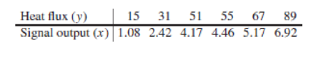
- a. Compute the least-squares line for predicting heat flux from the signal output.
- b. If the radiometer reads 3.00 V, predict the heat flux.
- c. If the radiometer reads 8.00 V, should the heat flux be predicted? If so, predict it. If not, explain why.
Want to see the full answer?
Check out a sample textbook solution
Chapter 7 Solutions
Statistics for Engineers and Scientists
Additional Math Textbook Solutions
Basic Business Statistics, Student Value Edition
Elementary Statistics: A Step By Step Approach
Introduction to Statistical Quality Control
Statistics for Business & Economics, Revised (MindTap Course List)
Introductory Statistics
An Introduction to Mathematical Statistics and Its Applications (6th Edition)


- Need help with (c) and (d) Mist (airborne droplets or aerosols) is generated when metal-removing fluids are used in machining operations to cool and lubricate the tool and workpiece. Mist generation is a concern to OSHA, which has recently lowered substantially the workplace standard. An article gave the accompanying data on x = fluid-flow velocity for a 5% soluble oil (cm/sec) and y = the extent of mist droplets having diameters smaller than 10 µm (mg/m3): x 88 177 182 354 369 442 970 y 0.39 0.60 0.50 0.66 0.61 0.69 0.92 (a) The investigators performed a simple linear regression analysis to relate the two variables. Does a scatter plot of the data support this strategy? (b) What proportion of observed variation in mist can be attributed to the simple linear regression relationship between velocity and mist? (Round your answer to three decimal places.) (c) The investigators were particularly interested in the impact on mist of increasing velocity from 100 to 1000 (a…arrow_forwardDescribe and compare the measurement of the central tendency and thedispersion of the electric usage before and after implementing the newelectric meter based on the histogram and box plots given.arrow_forwardAccumulation of mercury (Hg) in fish is hypothesized to correlate with the fish size. Barbonymus schwanenfeldii is a species commonly found in a dam in Sarawak. Table 1 shows data of Hg concentration (mg/kg) present in three sizes of fish caught in the dam in triplicates. (i, ii, iii was already answered.)arrow_forward
- Cell Phone Radiation Listed below are the measured radiation absorption rates (in W/kg) corresponding to these cell phones: iPhone 5S, BlackBerry Z30, Sanyo Vero, Optimus V, Droid Razr, Nokia N97, Samsung Vibrant, Sony Z750a, Kyocera Kona, LG G2, and Virgin Mobile Supreme. The data are from the Federal Communications Commission (FCC). The media often report about the dangers of cell phone radiation as a cause of cancer. The FCC has a standard that a cell phone absorption rate must be 1.6 W/kg or less. If you are planning to purchase a cell phone, are any of the measures of center the most important statistic? Is there another statistic that is most relevant? If so, which one?arrow_forwardCell Phone Radiation Listed below are the measured radiation absorption rates (in W/kg) corresponding to these cell phones: iPhone 5S, BlackBerry Z30, Sanyo Vero, Optimus V, Droid Razr, Nokia N97, Samsung Vibrant, Sony Z750a, Kyocera Kona, LG G2, and Virgin Mobile Supreme. The data are from the Federal Communications Commission.arrow_forwardThe article "Characteristics and Trends of River Discharge into Hudson, James, and Ungava Bays, 1964-2000" (S. Dery, M. Stieglitz, et al., Journal of Climate, 2005:2540-2557) presents measurements of discharge rate x (in kmlyr) andpeakflow y (in m/s) for 42 rivers that drain into the Hudson, James, and Ungava Bays. The data are shown in the following table: Discharge Peak Flow 94.24 4110.3 66.57 4961.7 59.79 10275.5 48.52 6616.9 40.00 7459.5 32.30 2784.4 31.20 3266.7 30.69 4368.7 26.65 1328.5 22.75 4437.6 21.20 1983.0 20.57 1320.1 19.77 1735.7 18.62 1944.1 17.96 3420.2 17.84 2655.3 16.06 3470.3 1561.6 14.69 11.63 869.8 11.19 936.8 11.08 1315.7 10.92 1727.1 9.94 768.1 7.86 483.3arrow_forward
- Aa Febru The body mass index (BMI) of a person is defined to be the person's body mass divided by the square of the person's height. The article "Influences of Parameter Uncertainties within the ICRP 66 Respiratory Tract Model: Particle Deposition" (W. Bolch, E. Farfan, et al., Health Physics, 2001:378-394) states that body mass index (in kg/m2) in men aged 25-34 is lognormally distributed with parameters u = 3.215 and o = 0.157. a.Find the mean and standard deviation BMI for men aged 25-34. b.Find the standard deviation of BMI for men aged 25-34. c.Find the median BMI for men aged 25-34. d.What proportion of men aged 25-34 have a BMI less than 20? e.Find the 80th percentile of BMI for men agėd 25 -34. 04... Rext 田arrow_forward17.7 Butterfly wings. Researchers studied the morphological attributes of monarch butterflies (Danaus plexippus), a species that undertakes large seasonal migrations over North America. They measured the forewing weight (in milligrams, mg) of a sample of 92 monarch butterflies, all of which had been reared in captivity in identical conditions.° Figure 17.4 shows the output from the statistical software JMP. (The data are also available in the Large.Butterfly the data file if you wish to practice working with your own software.) Estimate with 95% confidence the mean forewing weight of monarch butterflies reared in captivity. Follow the four- step process as illustrated in Example 17.2. 4 STEP そMP FWweight 30 25 20 15 10 11 12 13 14 15 8 9 10 Summary Statistics Mean 11.795652 Std Dev 1.1759413 Std Err Mean 0.1226004 Upper 95% Mean Lower 95% Mean 1 FIGURE 17.4 Software output (JMP) for the forewing weight of monarch 12.039183 11.552122 92 N. butterflies. Countarrow_forward#20 part b only- show full work for psych statsarrow_forward
- Foot ulcers are common problem for people with diabetes. Higher skin temperatures on the foot indicate an increased risk of ulcers. The article “An Intelligent Insole for Diabetic Patients with the Loss of Protective Sensation" (Kimberly Anderson, M.S. Thesis, Colorado School of Mines), reports measurements of temperatures, in °F, of both feet for 18 diabetic patients. The results are presented in the Table Q1. Table Ql: Measurements of temperatures, in °F of left foot Vs right foot for 18 diabetic patients Left Foot Right Foot Left Foot Right Foot 80 80 76 81 85 85 89 86 80 86 75 87 82 88 78 78 89 87 80 81 87 82 87 82 78 78 86 85 88 89 76 80 89 90 88 89 (d) Test the slope, ß1 = 1 at 5% level of significance. (e) Calculate the coefficient of correlation r and r2 and then interpret their valuesarrow_forwardPlease solve part d and e only. The body mass index (BMI) of a person is defined to be the person’s body mass divided by the square of the person’s height. The article “Influences of Parameter Uncertainties within the ICRP 66 Respiratory Tract Model: Particle Deposition” (W. Bolch, E. Farfan, et al., Health Physics, 2001:378–394) states that body mass index (in kg/m2) in men aged 25–34 is lognormally distributed with parameters μ = 3.215 and σ = 0.157. a.Find the mean and standard deviation BMI for men aged 25–34. b.Find the standard deviation of BMI for men aged 25–34. c.Find the median BMI for men aged 25–34. d.What proportion of men aged 25–34 have a BMI less than 20? e.Find the 80th percentile of BMI for men aged 25–34.arrow_forwardThe article "Mathematical Modeling of the Argon-Oxygen Decarburization Refining Process of Stainless Steel: Part II. Application of the Model to Industrial Practice" (J. Wei and D. Zhu, Metallurgical and Materials Transactions B, 2001:212-217) presents the carbon content (in mass %) and bath temperature (in K) for 32 heats of austenitic stainless steel. These data are shown in the following table. Carbon % Temp. 1975 19 23 1947 22 1954 16 1992 17 1965 18 1971 12 2046 24 1945 17 1984 20 1991arrow_forward
 MATLAB: An Introduction with ApplicationsStatisticsISBN:9781119256830Author:Amos GilatPublisher:John Wiley & Sons Inc
 Probability and Statistics for Engineering and th...StatisticsISBN:9781305251809Author:Jay L. DevorePublisher:Cengage Learning
 Statistics for The Behavioral Sciences (MindTap C...StatisticsISBN:9781305504912Author:Frederick J Gravetter, Larry B. WallnauPublisher:Cengage Learning
 Elementary Statistics: Picturing the World (7th E...StatisticsISBN:9780134683416Author:Ron Larson, Betsy FarberPublisher:PEARSON
 The Basic Practice of StatisticsStatisticsISBN:9781319042578Author:David S. Moore, William I. Notz, Michael A. FlignerPublisher:W. H. Freeman
 Introduction to the Practice of StatisticsStatisticsISBN:9781319013387Author:David S. Moore, George P. McCabe, Bruce A. CraigPublisher:W. H. Freeman