
Videos
RELATING CONCEPTS For Individual or Group Work (Exercises 91–94)
In 1935, Charles F. Richter devised a scale to compare the intensities of earthquakes. The intensity of an earthquake is measured relative to the intensity of a standard zero-level earthquake of intensity
For example, if an earthquake has magnitude 5.0 on the Richter scale, then its intensity is calculated as
which is 100,000 times as intense as a zero-level earthquake.
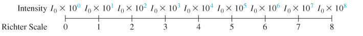
To compare two earthquakes, such as one that measures 8.0 to one that measures 5.0, calculate the ratio of their intensities.
An earthquake that measures 8.0 is 1000 time as intense as one that measures 5.0.
The table lists information for selected earthquakes with their years, locations, and magnitudes. Work Exercises 91–94 in order.
| Year | Earthquake Location | Richter Scale Measurement |
| 1960 | Chile | 9.5 |
| 1952 | Kamchatka | 9.0 |
| 2007 | Southern Sumatra, Indonesia | 8.5 |
| 2013 | Obihoro, Japan | 6.9 |
| 2002 | Hindu Kush, Afghanistan | 5.9 |
| Source: earthquake.usgs.gov | ||
Compare the intensity of the 2013 Obihoro earthquake with the 2002 Hindu Kush earthquake.
Want to see the full answer?
Check out a sample textbook solution
Chapter 4 Solutions
Beginning and Intermediate Algebra (6th Edition)


- part G Harrow_forwardQ1. The table provided gives data on indexes of output per hour (X) and real compensation per hour (Y) for the business and nonfarm business sectors of the U.S. economy for 1960–2005. The base year of the indexes is 1992 = 100 and the indexes are seasonally adjusted. a. Plot Y against X for the two sectors separately. b. What is the economic theory behind the relationship between the two variables? Does the scattergram support the theory? c. Estimate the OLS regression of Y on X. Note: on the table ( 1. Output refers to real gross domestic product in the sector. 2. Wages and salaries of employees plus employers’ contributions for social insurance and private benefit plans. 3. Hourly compensation divided by the consumer price index for all urban consumers for recent quarters.) Thank you!arrow_forwardQ. Table provided gives data on gross domestic product (GDP) for the United States for the years 1959–2005. a. Plot the GDP data in current and constant (i.e., 2000) dollars against time. b. Letting Y denote GDP and X time (measured chronologically starting with 1 for 1959, 2 for 1960, through 47 for 2005), see if the following model fits the GDP data: Yt = β1 + β2 Xt + ut Estimate this model for both current and constant-dollar GDP. c. How would you interpret β2? d. If there is a difference between β2 estimated for current-dollar GDP and that estimated for constant-dollar GDP, what explains the difference? e. From your results what can you say about the nature of inflation in the United States over the sample period?arrow_forward
- Energy consumption: The following table presents the average annual energy expenditures (in dollars) for housing units of various sizes (in square feet). Answer the question below.arrow_forwardStats #9.arrow_forwardThe scatterplot shows how the pulse rate changes with the weight of a person. Pulse Rate 86.41 - 0.09144(Weight) %3D 100 90 80 70 60 50 100 120 140 160 180 200 220 Pulse Ratearrow_forward
- Part D E Farrow_forwardThis question has several parts that must be completed sequentially. The following table shows total military and arms trade expenditure for a certain country in 2000, 2006, and 2012. Year t (year since 2000) 0 6 12 Military Expenditure C(t)($ billion) 40 270 510 (a) Compute and interpret the average rate of change of C(t) over the period 2006–2012 (that is, [6, 12]). Be sure to state the units of measurement. (b) Compute and interpret the average rate of change of C(t) over the period [0, 12]. Be sure to state the units of measurement. Recall that the average rate of change of f(x) over the interval [a, b] is the change in f divided by the change in x. The symbol Δ means "change in." average rate of change of f = change in f change in x = Δf Δx = f(b) − f(a) b − a Note that the given chart provides data points in the form of (t, C(t)). Year t (year since 2000) 0 6 12 Military Expenditure C(t)($ billion) 40 270 510 In the…arrow_forward1/2. Read and answer please this is a review questionarrow_forward
- e table below shows the life expectancy for an individu rs. ear of Birth Life Expectancy 930 59.7 940 62.9 950 70.2 965 69 7arrow_forward(3.1) #10arrow_forwardCell Phones Using the CTIA Wireless Survey for1985–2009, the number of U.S. cell phone subscribers (in millions) can be modeled byy = 0.632x2 - 2.651x + 1.209where x is the number of years after 1985.a. Graphically find when the number of U.S.subscribers was 301,617,000.b. When does the model estimate that the number ofU.S. subscribers would reach 359,515,000?c. What does the answer to (b) tell about this model?arrow_forward
 Algebra & Trigonometry with Analytic GeometryAlgebraISBN:9781133382119Author:SwokowskiPublisher:Cengage