
Videos
World Military Expenditure The following chart shows total military and arms trade expenditure from 1992–2010 (
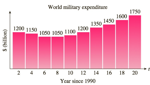
Source: www.globalissues.org/Geopolitics/ArmsTrade/Spending.asp.
a. If you want to model the expenditure figures with a function of the form
b. Which of the following models best approximates the data given? (Try to answer this without actually computing values.)
A.
B.
C.
D.
c. What is the nearest year that would correspond to the vertex of the graph of the correct model from part (b)? What is the danger of extrapolating the data in either direction?
Want to see the full answer?
Check out a sample textbook solution
Chapter 2 Solutions
Finite Mathematics and Applied Calculus (MindTap Course List)


- The Internal Revenue Service Restructuring and Reform Act (RRA) was signed into law by President Bill Clinton in 1998. A major objective of the RRA was to promote electronic filing of tax returns. The data in the table that follows show the percentage of individual income tax returns filed electronically for filing years 2000–2008. Since the percentage P of returns filed electronically depends on the filing year y and each input corresponds to exactly one output, the percentage of returns filed electronically is a function of the filing year;so P(y) represents the percentage of returns filed electronically for filing year y. (a) Find the average rate of change of the percentage of e-filed returns from 2000 to 2002. (b) Find the average rate of change of the percentage of e-filed returns from 2004 to 2006. (c) Find the average rate of change of the percentage of e-filed returns from 2006 to 2008. (d) What is happening to the average rate of change as time passes?arrow_forwardQ1. The table provided gives data on indexes of output per hour (X) and real compensation per hour (Y) for the business and nonfarm business sectors of the U.S. economy for 1960–2005. The base year of the indexes is 1992 = 100 and the indexes are seasonally adjusted. a. Plot Y against X for the two sectors separately. b. What is the economic theory behind the relationship between the two variables? Does the scattergram support the theory? c. Estimate the OLS regression of Y on X. Note: on the table ( 1. Output refers to real gross domestic product in the sector. 2. Wages and salaries of employees plus employers’ contributions for social insurance and private benefit plans. 3. Hourly compensation divided by the consumer price index for all urban consumers for recent quarters.) Thank you!arrow_forwardU.S. Population The number of White non-Hispanicindividuals in the U.S. civilian non-institutional population 16 years and older was 153.1 million in 2000and is projected to be 169.4 million in 2050.(Source: U.S. Census Bureau)a. Find the average annual rate of change in population during the period 2000–2050, with the appropriate units.b. Use the slope from part (a) and the population in2000 to write the equation of the line associatedwith 2000 and 2050.c. What does this model project the population to bein 2020?arrow_forward
- EXERCISE 1.3arrow_forwardQ. Table provided gives data on gross domestic product (GDP) for the United States for the years 1959–2005. a. Plot the GDP data in current and constant (i.e., 2000) dollars against time. b. Letting Y denote GDP and X time (measured chronologically starting with 1 for 1959, 2 for 1960, through 47 for 2005), see if the following model fits the GDP data: Yt = β1 + β2 Xt + ut Estimate this model for both current and constant-dollar GDP. c. How would you interpret β2? d. If there is a difference between β2 estimated for current-dollar GDP and that estimated for constant-dollar GDP, what explains the difference? e. From your results what can you say about the nature of inflation in the United States over the sample period?arrow_forwardproblen 1.4arrow_forward
- (3.7) #10arrow_forwardThe body mass index (BMI) of a person is the person’s weight divided by the square of his or her height. It is an indirect measure of the person’s body fat and an indicator of obesity. Results from surveys conducted by the Centers for Disease Control and Prevention (CDC) showed that the estimated mean BMI for US adults increased from 25.0 in the 1960–1962 period to 28.1 in the 1999–2002 period. [Source: Ogden, C., et al. (2004). Mean body weight, height, and body mass index, United States 1960–2002. Suppose you are a health researcher. You conduct a hypothesis test to determine whether the mean BMI of US adults in the current year is greater than the mean BMI of US adults in 2000. Assume that the mean BMI of US adults in 2000 was 28.1 (the population mean). You obtain a sample of BMI measurements of 1,034 US adults, which yields a sample mean of M = 28.9. Let μ denote the mean BMI of US adults in the current year. Please Formulate the null and alternative hypothesesarrow_forward
 Calculus For The Life SciencesCalculusISBN:9780321964038Author:GREENWELL, Raymond N., RITCHEY, Nathan P., Lial, Margaret L.Publisher:Pearson Addison Wesley,
 Algebra & Trigonometry with Analytic GeometryAlgebraISBN:9781133382119Author:SwokowskiPublisher:Cengage