Concept explainers
Videos
The following tables show the first-round winning scores of the NCAA men's and women's basketball teams.
TABLE 2-17 Men's Winning First-Round NCAA Tournament Scores
| 95 | 70 | 79 | 99 | 83 | 72 | 79 | 101 |
| 69 | 82 | 86 | 70 | 79 | 69 | 69 | 70 |
| 95 | 70 | 77 | 61 | 69 | 68 | 69 | 72 |
| 89 | 66 | 84 | 77 | 50 | 83 | 63 | 58 |
TABLE 2-18 Women's Winning First-Round NCAA Tournament Scores
| 80 | 68 | 51 | 80 | 83 | 75 | 77 | 100 |
| 96 | 68 | 89 | 80 | 67 | 84 | 76 | 70 |
| 98 | 81 | 79 | 89 | 98 | 83 | 72 | 100 |
| 101 | 83 | 66 | 76 | 77 | 84 | 71 | 77 |
Use the software or method of your choice to construct separate histograms for the men's and women's winning scores Try 5, 7, and 10 classes for each. Which number of classes seems to be the best choice? Why?
To graph: The histogram for men’s and women’s winning score data..
Explanation of Solution
Calculation: For Men’s winning score data:
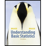
The largest value of the data set is 101 and the smallest value is 50 in the men’s winning score data.
Using five classes, the class width is calculated in the following way:
The frequency table is as follows:
| Class-limits | Class boundaries | Frequency |
| 50–60 | 49.5–60.5 | 2 |
| 61–71 | 60.5–71.5 | 13 |
| 72–82 | 71.5–82.5 | 8 |
| 83–93 | 82.5–93.5 | 5 |
| 94–104 | 93.5–104.5 | 4 |
To construct the histogram by using the MINITAB, the steps are as follows:
Step 1: Enter the class boundaries in C1 and frequency in C2.
Step 2: Go to Graph > Histogram > Simple.
Step 3: Enter C1 in Graph variable, then go to Data options > Frequency > C2.
Step 4: Click on OK.
The obtained histogram is
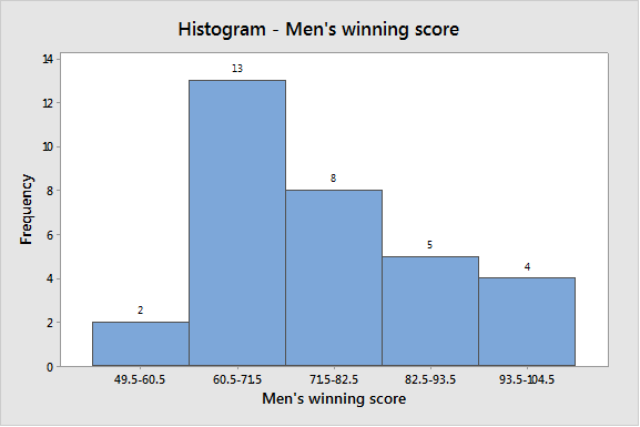
Using seven classes, the class width is calculated in the following way:
| Class-limits | Class boundaries | Frequency |
| 50–57 | 49.5–57.5 | 1 |
| 58–65 | 57.5–65.5 | 3 |
| 66–73 | 65.5–73.5 | 13 |
| 74–81 | 73.5–81.5 | 5 |
| 82–89 | 81.5–89.5 | 6 |
| 90–97 | 89.5–97.5 | 2 |
| 98–105 | 97.5–10.5 | 2 |
To construct the histogram by using the MINITAB, the steps are as follows:
Step 1: Enter the class boundaries in C3 and frequency in C4.
Step 2: Go to Graph > Histogram > Simple.
Step 3: Enter C3 in Graph variable, then go to Data options > Frequency > C4.
Step 4: Click on OK.
The obtained histogram is
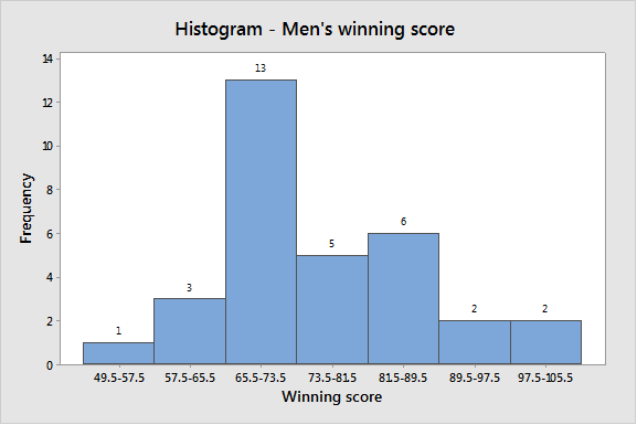
Using 10 classes, the class width is calculated in the following way:
| Class-limits | Class boundaries | Frequency |
| 50–55 | 49.5–55.5 | 1 |
| 56–61 | 55.5–61.5 | 2 |
| 62–67 | 61.5–67.5 | 2 |
| 68–73 | 67.5–73.5 | 12 |
| 74–79 | 73.5–79.5 | 5 |
| 80–85 | 79.5–85.5 | 4 |
| 86–91 | 85.5–91.5 | 2 |
| 92–97 | 91.5–97.5 | 2 |
| 98–103 | 97.5–103.5 | 2 |
| 104–109 | 103.5–109.5 | 0 |
To construct the histogram by using the MINITAB, the steps are as follows:
Step 1: Enter the class boundaries in C5 and frequency in C6.
Step 2: Go to Graph > Histogram > Simple.
Step 3: Enter C5 in Graph variable, then go to Data options > Frequency > C6.
Step 4: Click on OK.
The obtained histogram is
For Women’s winning score data:
The largest value of the data set is 101 and the smallest value is 51 in the women’s winning score data.
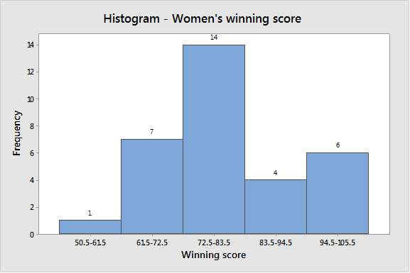
Using five classes, the class width calculated in the following way:
The frequency table is as follows:
| Class-limits | Class boundaries | Frequency |
| 51–61 | 50.5–61.5 | 1 |
| 62–72 | 61.5–72.5 | 7 |
| 73–83 | 72.5–83.5 | 14 |
| 84–94 | 83.5–94.5 | 4 |
| 95–105 | 94.5–105.5 | 6 |
To construct the histogram by using the MINITAB, the steps are as follows:
Step 1: Enter the class boundaries in C7 and frequency in C8.
Step 2: Go to Graph > Histogram > Simple.
Step 3: Enter C8 in Graph variable, then go to Data options > Frequency > C8.
Step 4: Click on OK.
The obtained histogram is
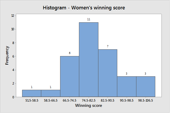
Using seven classes, the class width is calculated in the following way:
The frequency table is as follows:
| Class-limits | Class boundaries | Frequency |
| 51–58 | 51.5–58.5 | 1 |
| 59–66 | 58.5–66.5 | 1 |
| 67–74 | 66.5–74.5 | 6 |
| 75–82 | 74.5–82.5 | 11 |
| 83–90 | 82.5–90.5 | 7 |
| 91–98 | 90.5–98.5 | 3 |
| 99–106 | 98.5–106.5 | 3 |
To construct the histogram by using the MINITAB, the steps are as follows:
Step 1: Enter the class boundaries in C9 and frequency in C10.
Step 2: Go to Graph > Histogram > Simple.
Step 3: Enter C9 in Graph variable, then go to Data options > Frequency > C10.
Step 4: Click on OK.
The obtained histogram is:
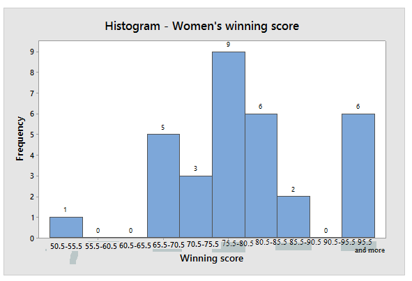
Using 10 classes, the class width calculated in the following way:
The frequency table is as follows:
| Class-limits | Class boundaries | Frequency |
| 51–55 | 50.5–55.5 | 1 |
| 56–60 | 55.5–60.5 | 0 |
| 61–65 | 60.5–65.5 | 0 |
| 66–70 | 65.5–70.5 | 5 |
| 71–75 | 70.5–75.5 | 3 |
| 76–80 | 75.5–80.5 | 9 |
| 81–85 | 80.5–85.5 | 6 |
| 86–90 | 85.5–90.5 | 2 |
| 91–95 | 90.5–95.5 | 0 |
| 96 and more | 95.5 and more | 6 |
To construct the histogram by using the MINITAB, the steps are as follows:
Step 1: Enter the class boundaries in C11 and frequency in C12.
Step 2: Go to Graph > Histogram > Simple.
Step 3: Enter C11 in Graph variable, then go to Data options > Frequency > C12.
Step 4: Click on OK.
The obtained histogram is
Using number classes five and seven in both data sets of men’s and women’s seem to be the best because histograms for that classes shows reliable distribution but using classes ten show gap between the bars. Since, using five classes seems best than using classes seven.
Want to see more full solutions like this?
Chapter 2 Solutions
Understanding Basic Statistics


- The following table gives the 2012 total payroll (in millions of dollars) and the percentage of games won during the 2012 season by each of the National League baseball teams. Total Payroll Тeam (millions of dollars) Runs Scored Arizona Diamondbacks 83 46 Atlanta Braves 89 35 Chicago Cubs 110 57 Cincinnati Reds 11 34 Colorado Rockies 93 39 Los Angeles Dodgers 264 51 Miami Marlins 59 38 Milwaukee Brewers 99 39 New York Mets 95 53 Philadelphia Phillies 127 33 Pittsburgh Pirates 82 58 San Diego Padres 92 40 San Francisco Giants 164 46 St. Louis Cardinals 112 59 Washington Nationals 156 45 The least squares regression line is u = 41.073 + 0.033x, where.x =total payroll (in millions of dollars) and y = percentage of games won. Predict the percentage of games won by a team with a total payroll of $87 million. Round your answer to the nearest integer.arrow_forwardMidterm and Final Exam Scores for 58 Business Statistics Students Midterm Exam Score Final Exam Score 80 78 87 85 72 81 69 54 86 70 83 73 78 89 75 84 74 86 75 79 84 75 73 63 74 72 73 69 80 86 75 78 72 75 77 68 76 77 66 78 74 77 71 73 85 79 74 74 76 79 76 73 84 72 77 81 78 86 86 76 81 83 78 83 85 86 73 71 83 83 83 79 72 68 83 90 84 89 73 83 86 81 76 79 58 58 73 77 81 85 72 67 77 70 82…arrow_forwardThe final grades in Basic Statistics of 80 students at Haramaya University are recorded in the accompanying table. 68 84 75 82 68 90 62 88 76 9373 79 88 73 60 93 71 59 85 7561 65 75 87 74 62 95 78 63 7266 78 82 75 94 77 69 74 68 6096 78 89 61 75 95 60 79 83 7179 62 67 97 78 85 76 65 71 7565 80 73 57 88 78 62 76 53 7486 67 73 81 72 63 76 75 85 77Use these data to prepare:(a) a frequency distribution.(b) a relative frequency distribution.(c) a cumulative frequency distributionarrow_forward
- The test scores of 32 students are listed below. Find Q3 32 37 41 44 46 48 53 55 56 57 59 63 65 66 68 69 70 71 74 74 75 77 78 79 80 82 83 86 89 92 95 99arrow_forwardListed below are the annual tuition amounts of the 10 most expensive colleges in a country for a recent year. What does this "Top 10" list tell us about the population of all of that country's college tuitions? $52,534 $51,382 $51,698 $51,867 $51,397 $53,988 $53,097 $51,212 $53,075 $51,397 ... Find the mean, midrange, median, and mode of the data set. The mean of the data set is $ . (Round to two decimal places as needed.)arrow_forwardFor each of the 32 National Football League teams, the numbers of points scored and allowed during the 2018 season are shown below. Team Wins Points Scored Points Allowed Team Wins PointsScored Points Allowed New York Jets 4 333 441 Chicago Bears 12 421 283 Cleveland Browns 7 359 392 Philadelphia Eagles 9 367 348 Denver Broncos 6 329 349 Tennessee Titans 9 310 303 Jacksonville Jaguars 5 245 316 Kansas City Chiefs 12 565 421 Minnesota Vikings 8 360 341 Baltimore Ravens 10 389 287 Oakland Raiders 4 290 467 Houston Texans 11 402 316 Cincinnati Bengals 6 368 455 Buffalo Bills 6 269 374 Washington Redskins 7 281 359 New Orleans Saints 13 504 353 Los Angeles Rams 13 527 384 Detroit Lions 6 324 360 Tampa Bay Buccaneers 5 396 464 Seattle Seahawks 10 428 347 Miami Dolphins 7 319 433 Indianapolis Colts 10 433 344 Pittsburgh Steelers 9 428 360 San Francisco 49ers 4 342 435 Green Bay Packers 6 376 400 Dallas Cowboys 10 339 324 New…arrow_forward
- The following is a chart of baseball players' salaries and statistics from 2016. Salary (in millions) Player Name RBI's HR's Miquel Cabrera 108 38 28.050 Yoenis Cespedes 86 31 27.500 Ryan Howard 59 25 25.000 Albert Pujols 119 31 25.000 Robinson Cano 103 39 24.050 Mark Teixeira 44 15 23.125 Joe Mauer 49 11 23.000 Hanley Ramirez Justin Upton 111 30 22.750 87 31 22.125 Adrian Gonzalez 90 18 21.857 Jason Heyward 49 7 21.667 Jayson Werth 70 21 21.571 Matt Kemp 108 35 21.500 Jacoby Ellsbury 56 9. 21.143 Chris Davis 84 38 21.119 Buster Posey 80 14 20.802 Shin-Soo Choo 17 7 20.000 Troy Tulowitzki Ryan Braun 79 24 20.000 91 31 20.000 Joey Votto 97 29 20.000 Hunter Pence 57 13 18.500 Prince Fielder 44 8 18.000 Adrian Beltre 104 32 18.000 Victor Martinez 86 27 18.000 Carlos Gonzalez 100 25 17.454 Matt Holliday 62 20 17.000 Brian McCann 58 20 17.000 Mike Trout 100 29 16.083 David Ortiz 127 38 16.000 Adam Jones 83 29 16.000 Curtis 59 30 16.000 Granderson Colby Rasmus 54 15 15.800 Matt Wieters 66 17…arrow_forwardEach year Money magazine publishes a list of "Best Places to Live in the United States." These listings are based on affordability, educational performance, convenience, safety, and livability. The below table shows the median household income of Money magazine’s top city in each U.S. state for (Money magazine website). City Median Household Income Pelham, AL $ 66,772 Juneau, AK $ 84,101 Paradise Valley, AZ $ 138,192 Fayetteville, AR $ 40,835 Monterey Park, CA $ 57,419 Lone Tree, CO $ 116,761 Manchester, CT $ 64,828 Hockessin, DE $ 115,124 St. Augustine, FL $ 47,748 Vinings, GA $ 73,103 Kapaa, HI…arrow_forwardThe test scores of 40 students are listed below find P 56 30 35 43 44 47 48 54 55 56 57 59 62 63 65 66 68 69 69 71 72 72 73 74 76 77 77 78 79 80 81 81 82 83 85 89 92 93 94 97 98arrow_forward
- Find P95 from the following data 1 5 8 14 21 22 23 25 26 28 30 31 34 39 40 42 43 49 53 56 59 62 64 69 72 75 77 78 79 81 83 92 94 97 100 P95 =arrow_forwardA survey of enrollment at 35 community colleges across the United States yielded the following figures†. 6414; 1550; 2109; 9350; 21828; 4300; 5944; 5722; 2825; 2044; 5481; 5200; 5853; 2750; 10012; 6357; 27000; 9414; 7681; 3200; 17500; 9200; 7380; 18314; 6557; 13713; 17768; 7493; 2771; 2861; 1263; 7285; 28165; 5080; 11622 Calculate the sample standard deviation. (Round your answer to one decimal place.)arrow_forwardThe following is a chart of 25 baseball players' salaries and statistics from 2016. Player Name RBI's HR's AVG Salary (in millions) Justin Turner 90 27 0.277 5.100 Leonys Martin 47 15 0.245 4.150 Hunter Pence 57 13 0.289 18.500 Brandon Crawford 84 12 0.275 6.000 Logan Forsythe 52 20 0.264 2.750 Adrian Gonzalez 90 18 0.285 21.857 Mike Trout 100 29 0.315 16.083 Prince Fielder 44 8 0.212 18.000 Victor Martinez 86 27 0.289 18.000 Buster Posey 80 14 0.288 20.802 Matt Wieters 66 17 0.243 15.800 Joey Votto 97 29 0.326 20.000 J.D. Martinez 68 22 0.307 6.750 Aaron Hill 38 10 0.262 12.000 Mark Teixeira 44 15 0.204 23.125 Shin-Soo Choo 17 7 0.242 20.000 Rajai Davis 48 12 0.249 5.950 Carlos Gonzalez 100 25 0.298 17.454 Hanley Ramirez 111 30 0.286 22.750 Troy Tulowitzki 79 24 0.256 20.000 Adam Jones 83 29 0.265 16.000 Denard Span 53 11 0.266 5.000 Matt Holliday 62 20 0.246 17.000 Brian McCann 58 20 0.242 17.000 Justin Upton 87 31 0.246 22.125…arrow_forward
 Holt Mcdougal Larson Pre-algebra: Student Edition...AlgebraISBN:9780547587776Author:HOLT MCDOUGALPublisher:HOLT MCDOUGAL
 Glencoe Algebra 1, Student Edition, 9780079039897...AlgebraISBN:9780079039897Author:CarterPublisher:McGraw Hill